Risk and return

Table of Contents

A. Risk and Return: Past and Prologue

I. Fundamentals Review

1. Expectation

In the scope of investments, expectation is the investors' forecast of different states of the economy in the future.

• Ex ante: Before the event.
  • Measures the expected return before the event.
• Ex post: After the event.
  • Measures the expected return after the event.

State of the economy	Probability	Return
Recession	20%	-5%
Normal	50%	5%
Expansion	30%	15%

$$\textbf{E(r)} = \Sigma_{s} \ p(s) \times [r_s]$$

Variance is an important measure of uncertainty. Gives a quantitative measure of how much realized deviates from what expected. This is also known as volatality.

$$\sigma^2 = \Sigma_{s} \ p(s) \times [r_s - \text{E(r)}]^2$$

2. Ex-post average returns & $\sigma$

Ex-post: After the fact, at t (today):

• Use the past to predict the future.
• Empirically, we use ex post (history) average returns to approximate ex ante expected returns.

Holding period return (HPR): Total return on an asset or investment portfolio over the period for which the asset or portfolio has been held.

$$\bar{r} = \Sigma^T_{t=1}\frac{\text{HPR}_t}{T}$$

Where, $T$ is number of observations and $\bar{r}$ is the average HPR.

Expost variance: $$\sigma^2 = \frac{1}{T-1} \Sigma_{i=1}^T (r_i-\bar{r})^2$$

Expost standard deviation: $$\sigma = \sqrt{\sigma^2}$$

Annualizing the statistics:

$$\bar{r}_{\text{annual}} = \bar{r}_p \times \text{periods} $$

$$\sigma_{annual} = \sigma_{period} \times \sqrt{\text{# periods}}$$

3. Normal distribution

In finance, we use the normal distribution to approximate the possible outcomes investors face.

• Risk is the difference between the expected return and the realized (actual) returns.

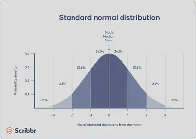
Normal distributions have key characteristics that are easy to spot in graphs:

1. The mean, median and mode are exactly the same.
2. The distribution is symmetric about the mean—half the values fall below the mean and half above the mean.
3. The distribution can be described by two values: the mean and the standard deviation.

Empirical rule

The empirical rule, or the 68-95-99.7 rule, tells you where most of your values lie in a normal distribution:

• Around 68.26% of values are within 1 standard deviation from the mean.
• Around 95.44% of values are within 2 standard deviations from the mean.
• Around 99.74% of values are within 3 standard deviations from the mean.

Value at Risk (VaR): The value at risk is the expected shortfall for a given confidence level.

• $E+(x)\sigma$ are the best cases
• $E-(x)\sigma$ are the worst cases

Hence, the attractiveness of an investment depends not just on the expected returns, but also the risk of losses.

II. Arithmetic vs. Geometric

When evaluating past performance, the geometric average is more precise in describing performance when volatility is high.

When statistically calculating expected returns using historical data, use simple average (Arithmetic) often because it is convenient, and it has nice statistical properties.

• Large sample theory: Sample size n grows indefinitely.
• Law of large numbers tells that the sample mean of a random variable converges to its true mean for a large sample.

III. Ex-ante Risk Premium & Risk Aversion

• Risk premium: The difference in expected return between risky and risk-free investments.

  • How much I would like to have at stake to be able to get high returns

  • Why do invester require it?

    • Investors are risk averse hence require a compensation to take on risk.
  • (aka) average excess return

• Risk-free rate $(r_f)$: Rate of return that can be earned with certainty.

B. Inflation and Real Rates of Return

Taxes are paid on nominal investment income. This reduces real investment income even further.

• nominal rate of return is amount of money generated by an investment before factoring in expenses such as taxes and inflation.

$$r_{\text{real}} \approx [r_{\text{nominal}}\times (1-\text{tax %})] - \text{Inflation rate}$$

C. Asset Allocation Across Risky and Risk-Free Portfolios

How much of your wealth should you invest in risky assets?

The amount you invest would depend on:

1. Risk
2. Risk premium - how much do investors get compensated for risk
3. Risk aversion - How much do investors dislike risk?

I. Complete Portfolio

The entire portfolio including risky portfolio (RP) and risk-free portfolio (RF).

$$E(r_{\text{complete}}) = yE(r_p) + (1-y)r_f$$

Risk-free asset, $r_f$: proxy with T-Bills/money market instruments.

$y$ is called the weight in the risky portfolio.

$$\sigma^2_{\text{complete}}=(y\sigma_{rp})^2 + [(1-y)\sigma_{\text{rf}}]^2$$

$\sigma_{\text{rf}}=0$ as the return from a risk-free asset is certain.

III. Capital Allocation Line (CAL)

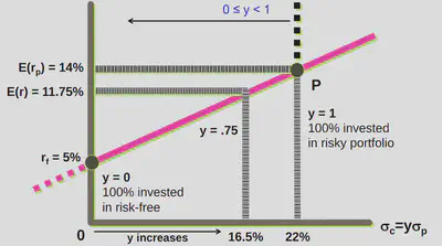
$$E(r_c) = r_f + \frac{\sigma_c}{\sigma_p}\times(E(r_p)-r_f)$$

The slope of the CAL measures the trade-off between risk ($\sigma_p$) and risk premium ($E[r_p]-r_f$).

The slope is known as the Sharpe ratio.

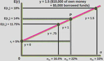
1. Using Leverage with CAL

Assumption: Borrow at risk-fre rate. (To ensure that the line is linear)

Borrow at the risk-free rate and invest in risky portfolio. With 50% leverage: $y=1.5$

Own money = $10,000

Borrowed money = $5,000

$$y=\frac{\text{own money}+\text{borrowed money}}{\text{own money}}$$

The line should be straight because for the following simple reasons.

• It could be kinked line if borrowing cost is higher than Rf.

IV. Risk Aversion and Allocation

Risk aversion is the willingness to trade off risk against expected return.

• Individual investors have different levels of risk aversion.

V. Quantifying Risk Aversion

Mean-variance analysis is one part of modern portfolio theory.

Assumption: Investors seek low risk and high reward.

• Variance may tell how spread out the returns of a specific security are on a daily or weekly basis.
• Expected return is a probability expressing the estimated return of the investment in the security.

$$A = \frac{E(r_c)-r_f}{\sigma_c^2}\gt0 \ \text{if risk adverse}$$

• Large A means that investor require additional return to bear risk

Average risk aversion = 1.5 to 4 (Empericallly)

A = 0; Risk neutral A < 0; Risk loving

$$y_{\text{percent in risky asset}} = \frac{(E(r_p)-r_f)/\sigma_p^2}{A_i}$$

D. Efficient Diversification

I. Asset Allocation With Two Risky Assets

1. Expected Return: Two Risky Assets

$$E(r_p) = W_1E_1(r_1)+W_2E(r_2)$$

2. Portfolio Variance and Standard Deviation: Two Risky Assets

$$\sigma^2_p = W_1^2\sigma^2_1 + W_2^2\sigma^2_2 + 2W_1W_2\text{Cov}(r_1,r_2)$$

$$Cov(R_A, R_B) = \frac{\Sigma_i^n(R_{A_i}-\bar{R_{A}})\times(R_{B_i}-\bar{R_{B}})}{n-1}$$

3. Relation between Covariance & Correlation Coefficient

• Correlation coefficient $\rho$

$$\rho_{1,2} = \frac{\text{Cov(r_1, r_2)}}{\sigma_1 \times \sigma_2}$$

• Correlation measures the intensity and direction that two stocks tend to move together

• Correlation is standardized to be between 1 and -1

4. Correlation Coefficient ($\rho_{1,2}$)

• If $\rho_{1,2}=1.0$ - Perfectly positively correlated

  • $\sigma(1,2) = W_1\sigma_1 + W_2\sigma_2$

Correlation is standardized to be between -1 and +1.

• If $\rho_{1,2}=-1.0$ - Perfectly negatively correlated
  • $\sigma(1,2) = \pm(W_1\sigma_1 - W_2\sigma_2$)

$$\sigma^2_p = W_1^2\sigma^2_1 + W_2^2\sigma^2_2 + 2W_1W_2\text{Cov}(r_1,r_2)$$

$$\text{Cov}(r_1, r_2)=\rho_{1,2}\sigma_1 \sigma_2$$

$$\sigma^2_p = W_1^2\sigma^2_1 + W_2^2\sigma^2_2 + 2W_1W_2\rho_{1,2}\sigma_1 \sigma_2$$