CAPM and APT (Part-1)
Table of Contents
A. Index Model & Capital Asset Pricing
I. Two Components of Stock Risk
$$\sigma_i^2 = \sigma^2(\alpha_i) + \sigma^2(\beta_iR_m) + \sigma^2(\epsilon_i)$$
Total risk = Systematic risk ($\sigma^2[\beta_iR_m]$) + Firm-specific risk ($\sigma^2[\epsilon_i]$)
-
$\sigma^2(\alpha_i) = 0$ Why? As $\alpha_i$ is the intercept hence does not change;
-
$var(\epsilon_i) = 0$? Not necessarily in index model, but yes in CAPM.
- In CAPM, we only invest in the market portfolio and it is fully diversified.
$R^2$ measures how much of the variation in $R_i$ is explained by $R_m$.
$R^2$ is fitness of the model.
$$R^2 = \frac{\beta_i^2 \sigma_m^2}{\sigma_i^2}$$
B. Capital Asset Pricing Model (CAPM)
The CAPM shows how risk and expected returns relate in equilibrium, and what type of investment risk matters.
Assumptions:
- Individual investors are “price takers”
- The trading does not affect the price
- Accept the price as given
- Investments are limited to traded finanicial assets
- No real estate, art, etc.
- No taxes or transaction costs
- Top bracket (22% for income > 320k)
- People only care about mean and variance of returns
- Strong assumption: People all have the same expectations, and the mean and variance of returns are known (Homogeneous expectations).
I. Overview of Implications
"All investors will hold some combination of the market portfolio (M) and the risk-rate"
Market portfolio:
- All assets of the security universe
- Market value weighted
- Optimal risky portfolio and on efficient frontier
CAPM, Capital Market Line
$$E[r_{C,M}] = r_f + y_M(E[r_M]-r_f)$$
Quick Recap
A theoretical concept that gives optimal combinations of a risk-free asset and the market portfolio.
The CML is superior to Efficient Frontier because it combines risky assets with risk-free assets.
Given all the assets have been invested in the risky portfolio (y=1), the market risk premium is:
$$E[r_M]-r_f = A\times\sigma_M^2$$
According to capital asset pricing model, the expected return of an asset is a linear function of the expected return of the market portfolio and risk-free rate.
$$E[r_{i}] = r_f + \beta_i(E[r_M]-r_f)$$
II. Understanding Beta
Beta is a measure of the systematic risk of a security relative to the market.
$$\beta_i = \frac{cov(r_i,r_M)}{\sigma_M^2}$$
- Beta is the sensitivity of a security’s excess return to the systematic factor (mkt risk premium).
III. Understanding alpha
Alpha measures how much expected returns differ from CAPM-implied expected returns.
$$\alpha = E(r_i) - r_f - \beta_i(E(r_M)-r_f)$$
- If $\alpha_i > 0$, then the security is underpriced and should be bought.
- If $\alpha_i < 0$, then the security is overpriced and should be short.
III. CAPM: Security Market Line
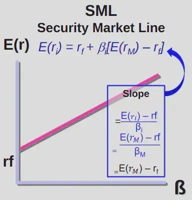
SML Slope is given by:
$$\frac{E[r_i]-r_f}{\beta_i} = \frac{E[r_m]-r_f}{\beta_m}$$
And $\beta_m = 1$, which gives us the CAPM equation.
C. Arbitrage Pricing Theory (APT)
I. Overview of APT
"Describes the relation between expected returns and risk when there are ONE or MORE sources of systematic risk."
A systematic risk must be:
-
Pervasive - Source of risk must potentially impact most companies, leading the stock prices to unexpcetedly change.
-
Undiversifiable - Source of risk can not be diversified away in a large portfolio.
II. APT: Assumptions
- No taxes, no transaction costs
- Investors can form well-diversified portfolios
- Well-diversified portfolios only contain systematic risk
- No arbitrage opportunities exist
Arbitrage: An investment strategy in which an investor simultaneously buys and sells an asset in different markets to profit from a difference in the price.
- An arbitrage opportunity exists when two securities always have the same payoff but DO NOT have the same price
D. How CML, CAPM, single index model and APT are related?
-
CML and CAPM: If the assumptions for cAP are true, the optimal risky portfolio becomes the market portfolio, and then we have CAPM.
-
Single index model is used to test the theories, for example, here CAPM, to see whether CAPM receives empirical support using data.
-
APT is another theoretical model to price the financial assets. It’s based on different assumptions. In week-2, you will see more of the differences with CAPM.
-
To test APT, we will introduce multi-factor models (empirical models).